 Zeb
Vance once suggested to me a link to an anemometer design, see
reference below. Here is my somewhat
modified
version
of that circuit: The temperature sensing elements are the base-emitter
junctions of two probe transistors
Q1, Q2. The base-emitter junction voltage is typically 0.7 Volts with a
temperature
coefficient near -2 mV per deg C. The lower transistor Q2 has its
collector wired to its base. This one acts as a passive diode,
only there to sense ambient temperature. These transistors form the
left side of a
bridge, the right side is resistors R1, R2, and the trimmer R3.
Amplifier A1 senses the balance of the bridge. If the voltage over the
Q1 junction is too high, then A1 will drive the Q1 base up. More
current will pass through both transistors but Q2 is fully conducting
and does not change its temperature appreciably with change in current.
Having a high collector voltage, Q1 will be heated while Q2
remains essentially at ambient temperature. That heating lowers the Q1
base-emitter voltage until balance is restored. The heater and the
temperature detection are inherent
in the transistor itself. So A1 keeps Q1 a certain number of degrees
hotter than Q2. How many depends on the trimmer setting, with this
circuit typically around 5 degrees centigrade. Resistor R4 senses how
much current is flowing through Q1-Q2. The (small)
voltage developed over R4 by this current is amplified by A2 into the
output pin 7. A2 has an offset input but otherwise simply translates
the additional current needed to maintain the temperature difference
between the two B-E junctions. The more current, the more heat is being
removed from hot Q2. Actually A2 is not simple at all. If R9 and R10
are trimmers, you can go nuts trying to adjust them. The reason is that
“input offset” in the front. As the bias changes, the gain is affected.
Zeb
Vance once suggested to me a link to an anemometer design, see
reference below. Here is my somewhat
modified
version
of that circuit: The temperature sensing elements are the base-emitter
junctions of two probe transistors
Q1, Q2. The base-emitter junction voltage is typically 0.7 Volts with a
temperature
coefficient near -2 mV per deg C. The lower transistor Q2 has its
collector wired to its base. This one acts as a passive diode,
only there to sense ambient temperature. These transistors form the
left side of a
bridge, the right side is resistors R1, R2, and the trimmer R3.
Amplifier A1 senses the balance of the bridge. If the voltage over the
Q1 junction is too high, then A1 will drive the Q1 base up. More
current will pass through both transistors but Q2 is fully conducting
and does not change its temperature appreciably with change in current.
Having a high collector voltage, Q1 will be heated while Q2
remains essentially at ambient temperature. That heating lowers the Q1
base-emitter voltage until balance is restored. The heater and the
temperature detection are inherent
in the transistor itself. So A1 keeps Q1 a certain number of degrees
hotter than Q2. How many depends on the trimmer setting, with this
circuit typically around 5 degrees centigrade. Resistor R4 senses how
much current is flowing through Q1-Q2. The (small)
voltage developed over R4 by this current is amplified by A2 into the
output pin 7. A2 has an offset input but otherwise simply translates
the additional current needed to maintain the temperature difference
between the two B-E junctions. The more current, the more heat is being
removed from hot Q2. Actually A2 is not simple at all. If R9 and R10
are trimmers, you can go nuts trying to adjust them. The reason is that
“input offset” in the front. As the bias changes, the gain is affected. It
is hard to understand the talk about linearity in the original
article until you realize it is stated for a rather small range, up to
250 ft/min, 1.27 m/s. I find from my calibrations in the 1 to 10 m/s
range
that the device is close to logarithmic, as seen here in the
calibration for a probe with TO-18 case transistors. Its output
voltage increases about equally much for each doubling of the air
speed. And this is also the kind of behavior one would like to have,
this largely obviates need for a range switch.
It
is hard to understand the talk about linearity in the original
article until you realize it is stated for a rather small range, up to
250 ft/min, 1.27 m/s. I find from my calibrations in the 1 to 10 m/s
range
that the device is close to logarithmic, as seen here in the
calibration for a probe with TO-18 case transistors. Its output
voltage increases about equally much for each doubling of the air
speed. And this is also the kind of behavior one would like to have,
this largely obviates need for a range switch.
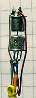
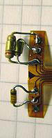
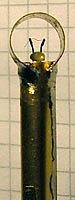
| This circuit remains with the principle of diode forward voltage temperature dependence, but now the hot diode is externally heated by a resistor. This diode was clamped to the heater with a tiny strip of brass sheet and also sealed to it with a drop of cyanoacrylate glue. The photo shows the probe tip cold and heated diodes. They are mounted on a flexible multiple conductor strip, retrieved from a head arm of a junked hard disk drive. The glass encapsulated 1N4448 diodes seem to have a fairly low thermal resistance, the data sheet says 0.24 K/mW including 10 mm leads. | |
 The
small voltage developed over R3 purports to govern the forward drop
difference, and hence the temperature difference between the diodes.
The
gain of the
balance sensing amplifier is by necessity moderated by the R5/R4
feedback network, together with a big slowing down capacitor C1.
There is a delay of heat transfer from the
heater to the heated diode. If the servo loop gain is too high, this
will make the circuit oscillate between fully on and off. The R6
heater resistor consumes more power than the bare amplifier can
deliver, so
an intermediate emitter follower transistor is added. The rather low
input voltage bias to the amplifier from the sensing diodes necessitate
D3
to increase the margin of amplifier negative supply.
The
small voltage developed over R3 purports to govern the forward drop
difference, and hence the temperature difference between the diodes.
The
gain of the
balance sensing amplifier is by necessity moderated by the R5/R4
feedback network, together with a big slowing down capacitor C1.
There is a delay of heat transfer from the
heater to the heated diode. If the servo loop gain is too high, this
will make the circuit oscillate between fully on and off. The R6
heater resistor consumes more power than the bare amplifier can
deliver, so
an intermediate emitter follower transistor is added. The rather low
input voltage bias to the amplifier from the sensing diodes necessitate
D3
to increase the margin of amplifier negative supply. This
circuit is simple, reliable, and sensitive. But one slight difficulty
may be to find a sufficiently low resistance thermistor such that it
can be driven enough hot at high speed, given the rather low supply
voltage. The alternative with R1=10k is for a very moderate temperature
rise, some 5K.
This
circuit is simple, reliable, and sensitive. But one slight difficulty
may be to find a sufficiently low resistance thermistor such that it
can be driven enough hot at high speed, given the rather low supply
voltage. The alternative with R1=10k is for a very moderate temperature
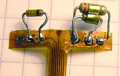
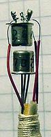
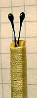
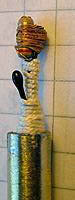
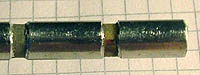
rise, some 5K.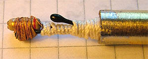 Also an externally heated version
was tried. The photo shows the probe with the hot NTC resistor lashed
with thin copper wire to the heater resistor. The original heater
resistor
leads are cut off and replaced by 0.24mm wire wrap leads to
reduce uncontrolled thermal leakage. The hot array is isolated from the
cold reference NTC resistor by a
lashing of sewing thread.
Also an externally heated version
was tried. The photo shows the probe with the hot NTC resistor lashed
with thin copper wire to the heater resistor. The original heater
resistor
leads are cut off and replaced by 0.24mm wire wrap leads to
reduce uncontrolled thermal leakage. The hot array is isolated from the
cold reference NTC resistor by a
lashing of sewing thread. This
circuit performs well, except for its inherent thermal delay between
heater and sensor. This necessitates
the slowing down feedback capacitor. Without it the circuit will
oscillate between on and off, with it the final reading is reached
after a prolonged delay, to the order of 30 seconds.
This
circuit performs well, except for its inherent thermal delay between
heater and sensor. This necessitates
the slowing down feedback capacitor. Without it the circuit will
oscillate between on and off, with it the final reading is reached
after a prolonged delay, to the order of 30 seconds.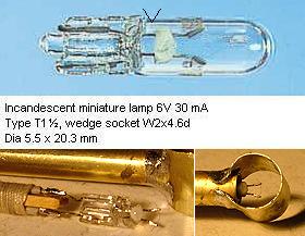 The hot wire anemometer is a
classical type and appears to
be the one
predominantly used for professional work. An orthodox such probe is
made
from Wollaston wire, a thin silver wire with a platinum core (priced
like US$ 500 for 8 inches of it). After soldering it to its posts under
a microscope you etch away the silver to leave a sub micrometer
diameter platinum wire. An exercise well beyond most amateurs.
The hot wire anemometer is a
classical type and appears to
be the one
predominantly used for professional work. An orthodox such probe is
made
from Wollaston wire, a thin silver wire with a platinum core (priced
like US$ 500 for 8 inches of it). After soldering it to its posts under
a microscope you etch away the silver to leave a sub micrometer
diameter platinum wire. An exercise well beyond most amateurs.  It must
be noted that without its bulb and inert atmosphere the
filament can not withstand anywhere near the original lamp
specification before being burned out. Be aware the lamp
cold resistance is 10-20 times lower than what is given by nominal
voltage and power. This particular lamp happens to
have
20 ohms cold resistance. For tungsten the resistive temp coefficient is
0.0045 /K such that the bridge balance value of 22 ohms is reached at
about 22 degrees centigrade temperature elevation. This is a very
moderate rise, such that correction will be necessary if ambient
temperature deviates appreciably from normal. Tweaking the fixed
resistor values in the bridge allows for some other temperature level.
On one hand R2 should be large enough to ensure the filament is never
burnt out. On the other hand R2 and supply voltage limit heating
current
such that there is a definite maximum measurable speed.
It must
be noted that without its bulb and inert atmosphere the
filament can not withstand anywhere near the original lamp
specification before being burned out. Be aware the lamp
cold resistance is 10-20 times lower than what is given by nominal
voltage and power. This particular lamp happens to
have
20 ohms cold resistance. For tungsten the resistive temp coefficient is
0.0045 /K such that the bridge balance value of 22 ohms is reached at
about 22 degrees centigrade temperature elevation. This is a very
moderate rise, such that correction will be necessary if ambient
temperature deviates appreciably from normal. Tweaking the fixed
resistor values in the bridge allows for some other temperature level.
On one hand R2 should be large enough to ensure the filament is never
burnt out. On the other hand R2 and supply voltage limit heating
current
such that there is a definite maximum measurable speed. To
get an air stream of known speed I used a vacuum cleaner, fed from a
variable transformer. That way the fan speed could be set arbitrarily
over some range. The cleaner hose was connected to a Venturi tube to
measure flow rate and the device ended with a nozzle where the probe
under test was placed centrally. To extend the measurement range I
could alternate between 22, 46
and 86 mm diameter nozzles. Knowing its diameter and
assuming a uniform air speed over its intake area A (m2) it
is
elementary to convert from flow Q (m3/s) into speed V (m/s):
V = Q/A. After running for a while the fan will heat the air passing
it. To avoid spurious effects from that, air was sucked from the
room rather than blown out from the nozzle.
To
get an air stream of known speed I used a vacuum cleaner, fed from a
variable transformer. That way the fan speed could be set arbitrarily
over some range. The cleaner hose was connected to a Venturi tube to
measure flow rate and the device ended with a nozzle where the probe
under test was placed centrally. To extend the measurement range I
could alternate between 22, 46
and 86 mm diameter nozzles. Knowing its diameter and
assuming a uniform air speed over its intake area A (m2) it
is
elementary to convert from flow Q (m3/s) into speed V (m/s):
V = Q/A. After running for a while the fan will heat the air passing
it. To avoid spurious effects from that, air was sucked from the
room rather than blown out from the nozzle. The flow meter
Venturi tube has two probe holes to measure the pressure drop from
input to constriction. By virtue of the Bernoulli law this drop is
proportional to the
square of the flow rate and was taken with a water U manometer, later
with a differential pressure transducer. The tube was calibrated by
measuring the time elapsed to fill a plastic bag of known volume. The
Venturi expands gradually after the constriction such that pressure is
partially regained. This has nothing to do with the flow measurement as
such, but it reduces the throttling effect of the meter.
The flow meter
Venturi tube has two probe holes to measure the pressure drop from
input to constriction. By virtue of the Bernoulli law this drop is
proportional to the
square of the flow rate and was taken with a water U manometer, later
with a differential pressure transducer. The tube was calibrated by
measuring the time elapsed to fill a plastic bag of known volume. The
Venturi expands gradually after the constriction such that pressure is
partially regained. This has nothing to do with the flow measurement as
such, but it reduces the throttling effect of the meter.| One would like to
know the temperature of the probe element. For the thermistor and hot
wire this is simple since the bridge
balance criterion (same resistance ratio both sides) tells about their
hot
electrical resistance. For those the temperature can then be computed
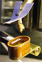
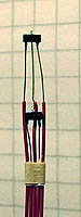
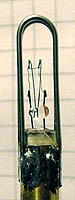
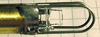
from their known cold resistance and the temperature coefficient. For a direct measurement I used a small oil filled container, carried on a digital thermometer probe. First the anemometer circuit was left to stabilize in still air and its output voltage was recorded. The container was heated with a soldering iron and was then left to cool down slowly while its temperature was tracked by the thermometer. At intervals the probe hot element was dipped into the oil. At the point where the anemometer output then stayed at its earlier recorded value, the oil temperature equals that of the probe tip. The small paper wing in the photo was to shield the cold reference sensor from hot air rising from the oil bath. |
|
 At left
is a generator that injects power P
(Watts) into
the circuit. C is
the thermal capacity of the device (e.g. transistor) measured in Joule
(Watt*seconds) per
degree (Kelvin or Centigrade), and the internal temperature of it
(junction temp) is To.
All
temperatures are relative to ambience = 'ground'.
At left
is a generator that injects power P
(Watts) into
the circuit. C is
the thermal capacity of the device (e.g. transistor) measured in Joule
(Watt*seconds) per
degree (Kelvin or Centigrade), and the internal temperature of it
(junction temp) is To.
All
temperatures are relative to ambience = 'ground'.
 External
heating eliminates the problem that heating power injection may
interfere with the temperature sensing. Here is what I figure is a
relevant though simplified thermal analogy
for an externally
heated probe. The sensor is enclosed in a separate
body, thermally connected to the heater by Ro which includes its
internal drop. Now there is a
distinction between the thermal capacity
Ch of the
heater and that of the sensor, Cs.
The Ro-Cs circuit makes a
low pass
filter that slows down operation and raises a stability problem to be
handled by the electrical feedback circuit. For instance, when Cs is being heated and
reaches the target temperature Ts,
then the circuit turns off power. Despite that, Cs will be even more
heated from the energy already stored in Ch.
External
heating eliminates the problem that heating power injection may
interfere with the temperature sensing. Here is what I figure is a
relevant though simplified thermal analogy
for an externally
heated probe. The sensor is enclosed in a separate
body, thermally connected to the heater by Ro which includes its
internal drop. Now there is a
distinction between the thermal capacity
Ch of the
heater and that of the sensor, Cs.
The Ro-Cs circuit makes a
low pass
filter that slows down operation and raises a stability problem to be
handled by the electrical feedback circuit. For instance, when Cs is being heated and
reaches the target temperature Ts,
then the circuit turns off power. Despite that, Cs will be even more
heated from the energy already stored in Ch. | Section |
1.1 | 1.1 | 1.1 | 1.1 | 1.2 | 1.3 | 1.4 | 1.5 | 1.5 | ||
 |
 |
 |
 |
 |
 |
 |
 |
 |
|||
| Quantity |
Symbol |
Dimension |
TO18
Cu leads |
TO18
Fe leads |
SOT23
Cu leads |
SOT23
Fe leads |
Ext Diode | NTC bridge | Ext NTC | Lamp
24V |
Lamp
6V 30mA |
| Int.
res. |
Ro | K/mW |
0,24 | 0,24 | 0,22 | 0,21 | 0,03 | 0,10 | 0,02 | 0,12 | 0,35 |
| Loss
res. |
Rl | K/mW | 0,09 | 0,13 | 0,07 | 0,55 | 0,12 | 0,24 | 0,19 | 2,18 | 6,90 |
| Cool
coeff. |
kRv | K(m/s)/mW |
0,15 | 0,09 | 0,47 | 0,30 | 0,11 | 0,38 | 0,25 | 1,06 | 7,43 |
| Temp.
rise |
dT | K |
30 | 39 | 29 | 32 | 5 | 5 | 7 | 20 | 22 |
| Error
|
E | % |
0,4 | 0,6 | 0,4 | 2,2 | 2,7 | 4,4 | 9,6 | 13,0 | 7,4 |
| Quality |
Rl/Ro | - |
0,4 | 0,5 | 0,3 | 2,7 | 4,6 | 2,3 | 11,4 | 19,0 | 19,6 |
| Mid
speed |
Vmed | m/s |
2,4 | 1,1 | 8,9 | 2,0 | 5,1 | 5,2 | 16 | 9,7 | 22 |
| Time const |
t |
s |
30 |
40 |
4 |
3 |
15 |
4 |
10 |
- |
- |
 |
This figure shows what indicator
meter scales would look like for the
various alternatives. They are derived from the actually measured
voltages and are expanded such that the range is from 0 to 20m/s. The
figures at left is the U voltage for the scale left end (0) in percent
of that for full scale (20). With the lower quality probes this offset
is rather high. These scales differ from the earlier theoretical examples since heating power and U are not directly proportional in the bottom five cases. I find no obvious explanation to why the scale for the NTC bridge comes so very close to an ideal logarithmic. |
| Photo |
Sect/Type |
Comment |
 |
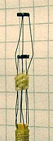
1.1 TO18 |
Rugged form with transistors potted inside an aluminum tube using Araldit two component epoxi. The increased masses and thermal resistances make the settling time several minutes. Sensitivity was reduced to about half, and it turned out bad in reproducing calibration. Looks nice, but is completely useless. |
 |
1.5 Lamp 12V 5W |
Halogen lamp. Cold resistance
less than 1 ohm requires additional power drive. |